Co-Induction and Term Graphs
Table of Contents
- 1. Introduction
- 2. Notation and basic definitions
- 3. Signature
- 4. Inductive terms
- 5. Term graphs
- 6. Inductive term graphs
- 7. Motivating Terms
- 8. (Co-Inductive) Terms
- 8.1. Observations and interactions
- 8.2. Position space
- 8.3. Behaviour
- 8.4. Composing Behaviours
- 8.5. Co-Inductive Terms as Behaviour
- 8.6. Subterm relation and rational terms
- 8.7. Observable behaviour of a vertex in a term graph
- 8.8. Example illustrating observable behaviour
- 8.9. Solution of a term graph
- 8.10. Proposition (Solution Lemma)
- 8.11. Co-Inductive terms as denotations of vertices in a term graph
- 8.12. Comparing inductive and co-inductive terms over a signature
- 8.13. Unique solution (from the theory of hypersets)
- 8.14. More examples
- 9. Reasoning about Equality of Terms via Bisimulation
- 10. Replacement
- 11. Implementing term graphs and replacement in Racket
- 12. Implementing Bisimulation for Rational terms
- 13. References
\( %% Your math definitions here % \newcommand{\alphaequiv}{{\underset{\raise 0.7em\alpha}{=}}} \newcommand{\yields}{\Rightarrow} \newcommand{\derives}{\overset{*}{\yields}} \newcommand{\alphaequiv}{=_{\alpha}} \newcommand{\tto}[2]{{\overset{#1}{\underset{#2}{\longrightarrow}}}} \newcommand{\transitsto}[2]{{\overset{#1}{\underset{#2}{\longrightarrow}}}} \newcommand{\xtransitsto}[2]{{\underset{#2}{\xrightarrow{#1}}}} \newcommand{\xtransitsfrom}[2]{{\underset{#2}{\xleftarrow{#1}}}} \newcommand{\xto}[2]{{\xtransitsto{#1}{#2}}} \newcommand{\xfrom}[2]{{\xtransitsfrom{#1}{#2}}} \newcommand{\xreaches}[2]{{\underset{#2}{\xtwoheadrightarrow{#1}}}} \newcommand{\reaches}[2]{{\underset{#2}{\xtwoheadrightarrow{#1}}}} %\newcommand{\reaches}[2]{{\overset{#1}{\underset{#2}{\twoheadrightarrow}}}} %\newcommand{\goesto}[2]{\transitsto{#1}{#2}} %\newcommand{\betareducesto}{{\underset{\beta}{\rightarrow}}} \newcommand{\betareducesto}{\rightarrow_{\beta}} %\newcommand{\etareducesto}{{\underset{\eta}{\rightarrow}}} \newcommand{\etareducesto}{\rightarrow_{\eta}} %\newcommand{\betaetareducesto}{{\underset{\beta\ \eta}{\rightarrow}}} \newcommand{\betaetareducesto}{\rightarrow_{\beta\eta}} \newcommand{\preducesto}{\rhd} \newcommand{\psimplifiesto}{\stackrel{\scriptstyle{*}}{\rhd}} \newcommand{\lreducesto}{\rightsquigarrow} \newcommand{\lsimplifiesto}{\stackrel{\scriptstyle{*}}{\lreducesto}} \newcommand{\rewritesto}{\hookrightarrow} \newcommand{\goesto}[1]{\stackrel{#1}{\rightarrow}} \newcommand{\xgoesto}[1]{\xrightarrow{#1}} \newcommand{\reducesto}{\stackrel{}{\rightarrow}} \newcommand{\simplifiesto}{\stackrel{\scriptstyle{*}}{\rightarrow}} \newcommand{\connected}[1]{\stackrel{#1}{\leftrightarrow}} \newcommand{\joins}{\downarrow} \newcommand{\evaluatesto}{\Longrightarrow} %\newcommand{\lit}[1]{\hbox{\sf{#1}}} \newcommand{\lit}[1]{{\sf{#1}}} \newcommand{\true}{\lit{true}} \newcommand{\false}{\lit{false}} \def\Z{\mbox{${\mathbb Z}$}} \def\N{\mbox{${\mathbb N}$}} \def\P{\mbox{${\mathbb P}$}} \def\R{\mbox{${\mathbb R}$}} \newcommand{\Rp}{{\mathbb{R}}^+} \def\Bool{\mbox{${\mathbb B}$}} \def\sA{\mbox{${\cal A}$}} \def\sB{\mbox{${\cal B}$}} \def\sC{\mbox{${\cal C}$}} \def\sD{\mbox{${\cal D}$}} \def\sF{\mbox{${\cal F}$}} \def\sG{\mbox{${\cal G}$}} \def\sL{\mbox{${\cal L}$}} \def\sP{\mbox{${\cal P}$}} \def\sM{\mbox{${\cal M}$}} \def\sN{\mbox{${\cal N}$}} \def\sR{\mbox{${\cal R}$}} \def\sS{\mbox{${\cal S}$}} \def\sO{\mbox{${\cal O}$}} \def\sT{\mbox{${\cal T}$}} \def\sU{\mbox{${\cal U}$}} \def\th{\mbox{$\widetilde{h}$}} \def\tg{\mbox{$\widetilde{g}$}} \def\tP{\mbox{$\widetilde{P}$}} \def\norm{\mbox{$\parallel$}} \def\osum{${{\bigcirc}}\!\!\!\!{\rm s}~$} \def\pf{\noindent {\bf Proof}~~} \def\exec{\mathit{exec}} \def\Act{\mathit{A\!ct}} \def\Traces{\mathit{Traces}} \def\Spec{\mathit{Spec}} \def\uns{\mathit{unless}} \def\ens{\mathit{ensures}} \def\lto{\mathit{leads\!\!-\!\!to}} \def\a{\alpha} \def\b{\beta} \def\c{\gamma} \def\d{\delta} \def\sP{\mbox{${\cal P}$}} \def\sM{\mbox{${\cal M}$}} \def\sA{\mbox{${\cal A}$}} \def\sB{\mbox{${\cal B}$}} \def\sC{\mbox{${\cal C}$}} \def\sI{\mbox{${\cal I}$}} \def\sS{\mbox{${\cal S}$}} \def\sD{\mbox{${\cal D}$}} \def\sF{\mbox{${\cal F}$}} \def\sG{\mbox{${\cal G}$}} \def\sR{\mbox{${\cal R}$}} \def\tg{\mbox{$\widetilde{g}$}} \def\ta{\mbox{$\widetilde{a}$}} \def\tb{\mbox{$\widetilde{b}$}} \def\tc{\mbox{$\widetilde{c}$}} \def\tx{\mbox{$\widetilde{x}$}} \def\ty{\mbox{$\widetilde{y}$}} \def\tz{\mbox{$\widetilde{z}$}} \def\tI{\mbox{$\widetilde{I}$}} \def\norm{\mbox{$\parallel$}} \def\sL{\mbox{${\cal L}$}} \def\sM{\mbox{${\cal M}$}} \def\sN{\mbox{${\cal N}$}} \def\th{\mbox{$\widetilde{h}$}} \def\tg{\mbox{$\widetilde{g}$}} \def\tP{\mbox{$\widetilde{P}$}} \def\norm{\mbox{$\parallel$}} \def\to{\rightarrow} \def\ov{\overline} \def\gets{\leftarrow} \def\too{\longrightarrow} \def\To{\Rightarrow} \def\points{\mapsto} %\def\yields{\mapsto^{*}} \def\un{\underline} \def\vep{$\varepsilon$} \def\ep{$\epsilon$} \def\tri{$\bigtriangleup$} \def\Fi{$F^{\infty}$} \def\Di{\Delta^{\infty}} \def\ebox\Box \def\emp{\emptyset} \def\leadsto{\rightharpoondown^{*}} \newcommand{\benum}{\begin{enumerate}} \newcommand{\eenum}{\end{enumerate}} \newcommand{\bdes}{\begin{description}} \newcommand{\edes}{\end{description}} \newcommand{\bt}{\begin{theorem}} \newcommand{\et}{\end{theorem}} \newcommand{\bl}{\begin{lemma}} \newcommand{\el}{\end{lemma}} %\newcommand{\bp}{\begin{prop}} %\newcommand{\ep}{\end{prop}} \newcommand{\bd}{\begin{defn}} \newcommand{\ed}{\end{defn}} \newcommand{\brem}{\begin{remark}} \newcommand{\erem}{\end{remark}} \newcommand{\bxr}{\begin{exercise}} \newcommand{\exr}{\end{exercise}} \newcommand{\bxm}{\begin{example}} \newcommand{\exm}{\end{example}} \newcommand{\beqa}{\begin{eqnarray*}} \newcommand{\eeqa}{\end{eqnarray*}} \newcommand{\bc}{\begin{center}} \newcommand{\ec}{\end{center}} \newcommand{\bcent}{\begin{center}} \newcommand{\ecent}{\end{center}} \newcommand{\la}{\langle} \newcommand{\ra}{\rangle} \newcommand{\bcor}{\begin{corollary}} \newcommand{\ecor}{\end{corollary}} \newcommand{\bds}{\begin{defns}} \newcommand{\eds}{\end{defns}} \newcommand{\brems}{\begin{remarks}} \newcommand{\erems}{\end{remarks}} \newcommand{\bxrs}{\begin{exercises}} \newcommand{\exrs}{\end{exercises}} \newcommand{\bxms}{\begin{examples}} \newcommand{\exms}{\end{examples}} \newcommand{\bfig}{\begin{figure}} \newcommand{\efig}{\end{figure}} \newcommand{\set}[1]{\{#1\}} \newcommand{\pair}[1]{\langle #1\rangle} \newcommand{\tuple}[1]{\langle #1\rangle} \newcommand{\union}{\cup} \newcommand{\Union}{\bigcup} \newcommand{\intersection}{\cap} \newcommand{\Intersection}{\bigcap} \newcommand{\B}{\textbf{B}} %\newcommand{\be}[2]{\begin{equation} \label{#1} \tag{#2} \end{equation}} \newcommand{\abs}[1]{{\lvert}#1{\rvert}} \newcommand{\id}[1]{\mathit{#1}} \newcommand{\pfun}{\rightharpoonup} %\newcommand{\ra}[1]{\kern-1.5ex\xrightarrow{\ \ #1\ \ }\phantom{}\kern-1.5ex} %\newcommand{\ras}[1]{\kern-1.5ex\xrightarrow{\ \ \smash{#1}\ \ }\phantom{}\kern-1.5ex} \newcommand{\da}[1]{\bigg\downarrow\raise.5ex\rlap{\scriptstyle#1}} \newcommand{\ua}[1]{\bigg\uparrow\raise.5ex\rlap{\scriptstyle#1}} % \newcommand{\lift}[1]{#1_{\bot}} \newcommand{\signal}[1]{\tilde{#1}} \newcommand{\ida}{\stackrel{{\sf def}}{=}} \newcommand{\eqn}{\doteq} \newcommand{\deduce}[1]{\sststile{#1}{}} %% \theoremstyle{plain}%default %% \newtheorem{thm}{Theorem}[section] %% \newtheorem{lem}[thm]{Lemma} %% \newtheorem{cor}[thm]{Corollary} %% % %% \theoremstyle{definition} %% \newtheorem{defn}[thm]{Definition} %% % %% \theoremstyle{remark} %% \newtheorem{remark}[thm]{Remark} %% \newtheorem{exercise}[thm]{Exercise} %% See http://u.cs.biu.ac.il/~tsaban/Pdf/LaTeXCommonErrs.pdf %% \newtheorem{prop}[thm]{Proposition} \newcommand{\less}[1]{#1_{<}} \newcommand{\pfn}{\rightharpoonup} \newcommand{\ffn}{\stackrel{{\sf fin}}{\rightharpoonup}} \newcommand{\stkout}[1]{\ifmmode\text{\sout{\ensuremath{#1}}}\else\sout{#1}\fi} % \DeclareMathSymbol{\shortminus}{\mathbin}{AMSa}{"39} \newcommand{\mbf}[1]{\mathbf{#1}} \)
1 Introduction
Recall the notion of finite, or inductively defined terms. Each inductively defined term may be identified by a tree. In this writeup, we revisit terms in a more general setting here, one that includes both finite and infinite terms, represented by not only trees but (finite or infinite) graphs. These more general terms are known by different names: co-inductive terms, coterms, or term graphs. We will use these names interchangeably.
The study of co-inductive terms may be approached from multiple mathematical perspectives. They may be seen final co-algebras in category theory. They may be interpreted as the largest fixed points of a signature operator. They can also be thought of as non-well-founded sets in non-well-founded set theory. They may be interpreted as finite or infinite labeled directed graphs. The approach we take here is to connect terms with behaviour expressed as a function that maps a sequence of interactions to an observation that is closely related to their graphical representation. This approach is attractive for two reasons: first, it builds on material that you are already familiar with: graphs and functions. Second, it interprets terms as interactive abstract machines. The notion of a machine (and its manifestation as an interpreter) is central to the operational approach to programming language semantics. Finally, interaction brings these abstract machines to life: a program is run by interacting with a machine that executes it.
2 Notation and basic definitions
2.1 Currying
For the sake of clarity, we will use curried notation for function application. \(f(x)\) will frequently be written as \(f\ x\) and \(f\ x\ y\) or \(f(x)(y)\) will mean \((f(x))(y)\). Occasionally, this could lead to ambiguity, e.g., when we wish to represent \(x\ y\) as the concatenation of \(x\) and \(y\). In such cases, ambiguity will be resolved by clarification of the specific use.
2.2 Set membership
The Colon symbol \((:)\) will be used interchangeably with \(\in\) to denote membership: \(x:A\) is identical to \(x\in A\).
2.3 Index and positions
\(\N\) denotes the set of natural numbers. \(\N_1\) denotes the set of positive natural numbers. An index is a positive natural number. Let \(m:\N\) denote a natural number. \(\N_1(m)\) denotes the subset of \(\N_1\) consisting of indices less than or equal to \(m\). Note that \(\N_1(0)\) is empty.
2.4 Partial Functions
If \(f:A\pfn B\) is a partial function from \(A\) to \(B\), then \(A\) and \(B\) are called the domain and the codomain of \(f\) and denoted \(\id{dom}\ f\) and \(\id{cod}\ f\), respectively. The domain of definition of \(f\), written \(\id{dod}\ f\) is the set \({x\in A\ |\ \exists y\in B. y=f\ x}\). The range of \(f\), denoted \(\id{rng}\ f\) is the set of all \(y\in B\) such that there is an \(x\in A\) such that \(f\ x=y\).
3 Signature
3.1 Signature
A signature \(\Sigma\) is a finite set of constructor symbols along with an arity function \(\alpha:\Sigma\rightarrow \N\). We write \(\Sigma^{(n)}\) to denote the set of all constructors that have arity \(n\). A constructor is said to be nullary if its arity is zero.
3.2 An example signature
3.2.1 Example signature
Consider the example signature \(\Sigma = \set{{\sf a}, {\sf g}, {\sf f}}\) with \(\alpha({\sf a})=0\) and \(\alpha({\sf g})=1\) and \(\alpha({\sf f})=2\). We will use this signature for the examples in this lesson.
3.2.2 Racket implementation of example signature
In a Racket implementation, each constructor is simply functions that create lists consisting of a head symbol and other arguments. We call the results of the construction as terms.
(define (a) (list 'a))
(define (b) (list 'b))
(define (g t) (list 'g t))
(define (f t1 t2) (list 'f t1 t2))
4 Inductive terms
4.1 Definition
The set of \(T_{\sf ind}(\Sigma)\) of inductive terms over a signature \(\Sigma\) is defined using the following rule \[ \frac{\tau_1:T_{\sf ind}(\Sigma)\quad \ldots \quad \tau_n:T_{\sf ind}(\Sigma)} {f(\tau_1, \ldots, \tau_n)\ : T_{\sf ind}(\Sigma)} \quad f:\Sigma^{(n)}\qquad CONS \]
Recall that a rule tells us how to derive new judgements from old. A rule consists of a consequent and antecedent parts:
- A consequent which is the concluding judgement (written below the line).
- A set of antecedent judgements (written above the line).
In addition, a rule may have side conditions, which are written immediately to the right of the rule. A rule also has a name, for reference, which is written left most to the rule.
Exercise: Identify all the pieces of the rule above.
If each of the antecedent judgements is derivable, and the side conditions hold, then the consequent judgement is derivable using the given rule.
The structure \(f(\tau_1, \ldots, \tau_n)\) is a more traditional syntax for the list \((f, \tau_1, \ldots, \tau_n)\). We will continue to use the former notation in our narrative, but switch to the latter (sans commas!) when implementing terms in Racket.
The inductive terms \(\tau_1, \ldots \tau_n\) are called immediate subterms of \(f(\tau_1, \ldots, \tau_n)\). The transitive closure of the immediate subterm relation is the proper subterm relation.
4.2 Well-foundedness property
It is not possible to have an inductive term \(\tau\) such that \(\tau\) is a proper subterm of itself. (Exercise: prove it).
5 Term graphs
5.1 Term Graph
Let \(\N_1\) denote the set of positive integers. A term graph over a signture \(\Sigma\) is a tuple \(\pair{V, h, \xto{}{}}\) where
- \(V\) is a (countable) set of vertices.
- \(h\) is the head function mapping \(V\) to \(\Sigma\).
- \(\xto{}{} \subseteq V\times \N_1\times V\) is a transition relation. We write \((v, i, v')\) as \(v\xto{i}{}v'\). We say that \(i\) takes \(v\) to \(v'\).
- If \(h(v)\in \Sigma^{(n)}\), then \(v\) has exactly \(n\) out-edges. For each \(i\), \(1\leq i \leq n\), there is exactly one out-edge labeled \(i\).
5.2 Reachability and Destination
Assume a term graph \(G\) with vertices \(v\) and \(v'\). Let \(p\) denote an index sequence. \(v\xto{p}{G}{v'}\) means that there is a path from \(v\) to \(v'\) whose label is \(p\). We say that \(p\) takes \(v\) to \(v'\). Another way of saying this is that \(v'\) is reachable from \(v\) via \(p\).
The path relation may be defined inductively.
\begin{align*} \frac{}{v\xto{[\ ]}{G}v} & \qquad\qquad \text{REF}\\ \\ \frac{v_i\xto{p}{G}v'}{v\xto{[i\ .\ p]}{G}v'}\quad v\xto{i}{G}v_i & \qquad \text{TRANS} \end{align*}It is not hard to see that since \(G\) is a term graph, \(v\xto{p}{G}r\) is in fact a function: if \(v\xto{p}{G}s\), then \(r=s\). (Exercise: prove this.)
If \(v\) is a vertex in a term graph \(G\), then \(\id{pos}_G\ v\) denotes the set of positions for \(v\), i.e., the set of all index sequences \(p\) such that \(v\xto{p}{G}v'\) for some vertex \(v'\) in \(G\). \(\id{dest}_G\ v\) maps a position in \(\id{pos}_G\ v\) to the unique vertex that is reachable from \(v\) via \(p\). We drop the subscript \(G\) when it is clear from the context.
5.3 Term graph as a Flat System of Equations
If \(h(v)=f\) and \(f\in \Sigma^{(n)}\) and \(v\xto{i}{G}v_i\), for each \(i:1\leq i\leq n\), then we denote this by the relation
\[v \eqn f(v_1, \ldots, v_n)\]
to indicate that (a) \(\id{h}(v)=f\), (b) \(f\in \Sigma^{(n)}\), and (c) for each \(i\) \(1\leq i\leq n\), \(v\xto{i}{G}v_i\).
The above looks like an equation if we interpret the vertices as variables. In particular, the relation element is a `flat term equation', `flat' because the constructor is applied to other vertices. A term graph may be completely specified by a system of such `flat term equations' with one equation for each vertex in the term graph.
6 Inductive term graphs
A term graph \(G\) is inductive if it is finite and acyclic. There is a hierarchy (non-circular relationship) between vertices.
6.1 Solution
A solution to an inductive term graph over \(\Sigma\) is a map \(\sigma\) from \(V_G\) to inductive terms over \(\Sigma\) that `solves' the flat system of equations: i.e., for each `flat equation' \(v \eqn f(v_i, \ldots, v_n)\) in \(G\):
\[\sigma\ v = f(\sigma\ v_1, \ldots, \sigma\ v_n)\]
6.2 Example
The inductive term graph \(G\) and its representation as a system of equations is shown below:
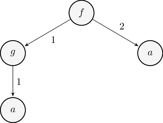
6.2.1 Solution to \(G\)
The following map solves \(G\). (Exercise. Verify this.)
\begin{align*} t_1 &\mapsto {\sf f(g(a), a)}\\ t_2 &\mapsto {\sf g(a)}\\ t_3 &\mapsto {\sf a}\\ t_4 &\mapsto {\sf a} \end{align*}6.2.2 Racket implementation of solution
In Racket, the solution is automatically based on Racket's
implementation of inductive terms and its evaluation
process. The Racket keyword let* is a shortcut for nested
let expressions.
(let* ([t4 (a)]
       [t3 (a)]
       [t2 (g t4)]
       [t1 (f t2 t3)])
  (check-false (eq? t3 t4))
  (check-equal? t1 '(f (g (a)) (a))))
We can clearly see that inductive terms are just nested lists whose head element is a constructor symbol and whose remaining elements if any are also inductive terms.
6.3 Proposition: Every inductive term graph has a unique solution
Proof: left as an exercise.
7 Motivating Terms
7.1 Inductive terms are solutions for inductive term graphs
So far, we have seen inductive terms and term graphs. We have seen that each vertex of an inductive term graph may be interpreted as a inductive term.
7.2 Inductive terms can not be solutions for cyclic term graphs
But what about terms graphs that are not inductive? For such graphs, the notion of solution based on inductive terms we have defined so far no longer holds:
Consider for example the equation representing the cyclic term graph \(G\) below.
\begin{align*} t &\eqn {\sf g}(t) \end{align*}Let \(\sigma = \set{t\mapsto \tau}\) where \(\tau\) is an inductive term. Suppose \(\sigma\) is a solution of \(G\). Then, we should have
\begin{align*} \sigma(t) &= {\sf g}(\sigma(t)), \qquad \text{or}\\ \tau &= {\sf f}(\tau) \end{align*}Clearly \(\tau\) does not exist, as this violates the well-foundedness property of inductive terms. Therefore, for cyclic term graphs can not have solutions that consist only of inductive terms. But can they have solutions that are not inductive `terms'? This begs the question of what is a `term', after all?
8 (Co-Inductive) Terms
8.1 Observations and interactions
We wish to associate a term with each vertex in a term graph but we are grappling with the question of what is a term. One way to answer to this question is to consider what we can observe at the vertex and how we can `interact' with it. The observation related to a vertex is simply its head. A `unit' interaction consists of supplying an index (between 1 and the arity of the vertex's head) to the vertex and getting back another vertex (the child).
Notice that we can overload the equation to mean the following:
- An observation that the head of \(v\) is \(f\) and
- \(n\) unit interactions with \(v\) that respectively yield the vertices \(v_1, \ldots, v_n\).
is literally the relation \(v \eqn f(v_1, \ldots, v_n)\).
8.2 Position space
A position space is any set of index sequences \(P\) that that is prefix closed: if \(q\in P\) then every prefix \(p\) of \(q\) is also in \(P\).
8.2.1 Position space of a vertex in a term graph
The set of positions \(\id{pos}_G\ v\) of a vertex \(v\) in a term graph \(G\) forms a position space. (Exercise: verify this.)
8.2.2 Example of a position space
In Example 6.2, the position space \(\id{pos}(t_1)\) associated with the vertex \(t_1\) is the set of positions \(\set{[\ ], [1], [2], [1\ 1]}\).
8.3 Behaviour
8.3.1 Behaviour over a signature
A behaviour \(B\) over a signature \(\Sigma\) is a total function from a position space (denoted \(\id{pos}_G\ B\)) to \(\Sigma\) that is upward closed, i.e.,
If \(p\) is a position in \(B\), and \(B\ p\) is a constructor of arity \(n\), then
- If \(i\) is a positive integer between \(1\) and \(n\), then \(pi\) is a position in the position space of \(B\), and
- If \(i\) is a positive integer and \(pi\) is in the position space of \(B\), then \(1\leq i\leq n\).
Here, \(pi\) denotes the concatenation of the position \(p\) with the index \(i\).
One way to think about behaviour is that positions identify the possible interactions that need to be done before an observation can be made. The `upward closed' property is to imagine that if we are at a position from where we can observe a constructor with arity \(n\), then there are exactly \(n\) possible `interactions' at that position. Since each interaction is identified with a position, this means that each \(pi\), where \(i\), \(1\leq i \leq n\) is also an interaction. Conversely, if \(pi\) is an interaction, then \(1\leq i \leq n\).
8.3.2 The concatenation of an index with a behaviour
If \(B\) is a behaviour over \(\Sigma\) and \(i\in\N_1\), then \(i\ B\) is the map defined as follows:
\[i\ B \ida \set{(ip \mapsto B\ p)\ |\ p\in \id{pos}_G\ B}\]
Exercise: Is \(i\ B\) a behaviour? Justify your answer.
8.3.3 Examples of behaviours
Assume \(\Sigma\) has constructors \({\sf f}, {\sf g}, {\sf a}, {\sf b}\) with arity 2, 1, 0, and 0 respectively. Then, The following maps are all behaviours:
\begin{align*} B_1 &\ida \set{[\ ]\mapsto {\sf a}}\\ B_2 &\ida \set{[\ ]\mapsto {\sf b}}\\ B_3 &\ida 1\ B_1 \union \set{[\ ]\mapsto {\sf g}}\\ B_4 &\ida 1\ B_3 \union 2\ B_2 \union \set{[\ ]\mapsto {\sf f}} \end{align*}8.4 Composing Behaviours
If \(B_1\ldots B_n\) are behaviours and \(f\in \Sigma^{(n)}\), then we write \(f(B_1\ldots, B_n)\) to denote the behaviour \((\Union_{i=1}^n\ i\ B_i) \union \set{[\ ]\mapsto f}\).
8.4.1 Example
Using this notation, the behaviours of Example 8.3.3 may be rewritten as compositions:
\begin{align*} B_1 &\ida {\sf a}()\\ B_2 &\ida {\sf b}()\\ B_3 &\ida {\sf g}(B_1)\\ B_4 &\ida {\sf f}(B_3, B_2) \end{align*}8.5 Co-Inductive Terms as Behaviour
Now, we are ready to formally define a term:
Defn [(Co-Inductive) Term] Given a signature \(\Sigma\) a term over \(\Sigma\) is a behaviour over \(\Sigma\).
Notice that in the definition of term, we have dispensed with the notion of vertices or term graphs. The notion of a term exists independent of a term graph, but may be generated via interactions with a vertex in a term graph.
(Co-Inductive) terms are behaviours over a signature. A term is inductive if its domain of definition is a finite position space.
Exercise: Verify that the definition of inductive terms via derivation using the CONS rule matches the above characterization.
8.6 Subterm relation and rational terms
Let \(t\) and \(t_i\) be two terms. \(t_i\) is an immediate subterm of \(t\) if there exists an \(f\in \Sigma\) and terms \(t_1, \ldots, t_n\) such that
- \(t = f(t_1,\ldots, t_n)\) and
- \(t'=t_i\) for some \(i\), \(1\leq i\leq n\).
The reflexive transitive closure of the immediate subterm relation is called the subterm relation. A term is rational if the set of all its subterms is finite.
8.7 Observable behaviour of a vertex in a term graph
One way of capturing the sum total of interactions and observations at a vertex is to list (a) the set of all valid interaction sequences (positions), and (b) and the observation of the head of the destination vertex at the end of each path. We call this the observable behaviour, or just behaviour of a vertex.
Formally, let \(G\) be a term graph over a signature \(\Sigma\). The observable behaviour of a vertex \(v\) in \(G\), written \(\id{obs}_G\ v\), is a map from the position space \(\id{pos}_G\ v\) to \(\Sigma\) and is defined as
\[\id{obs}_G\ v\ p \ida h(\id{dest}_G\ v\ p)\]
The following inductive definition is an alternative way to define the observable behaviour function:
\begin{align*} \frac{}{\id{obs}\ v\ [\ ] = h(v)} & \qquad\qquad \text{REF}\\ \\ \frac{\id{obs}\ v_i\ p = f}{\id{obs}\ v\ ip = f}\quad v\xto{i}{G}v_io & \qquad \text{TRANS} \end{align*}(Exercise: show that the two alternative definitions are equivalent.)
\(\id{obs}_G\) is called the observable behaviour map of term graph \(G\). The range of \(\id{obs}_G\), denoted \({\cal B}_G\) is called the set of observable behaviours in \(G\).
8.8 Example illustrating observable behaviour
Let us revisit the term graph \(G\) of Example 6.2, For the vertex \(t_1\), its position space is the set \(\set{[\ ], [1], [2], [1\ 1]}\). Its observable behaviour, \(\id{obs}(t_1)\), is the map
\begin{align*} [\ ] & \mapsto {\sf f}\\ [1] & \mapsto {\sf g}\\ [2] & \mapsto {\sf a}\\ [1\ 1] & \mapsto {\sf a} \end{align*}The set of observable behaviours of \(G\) is the collection of observable behaviours of each of its vertices.
\begin{align*} {\cal B}_G &= \id{obs}(t_1) \union &= \set{[\ ] \mapsto {\sf f}, [1]\mapsto {\sf g}, [2]\mapsto {\sf a}, [1\ 1]\mapsto {\sf a}} \union\\ &= \id{obs}(t_2) \union &= \set{[\ ] \mapsto {\sf g}, [1]\mapsto {\sf a}} \union\\ &= \id{obs}(t_3) \union &= \set{[\ ] \mapsto {\sf a}}\union\\ &= \id{obs}(t_4) &= \set{[\ ] \mapsto {\sf a}} \end{align*}8.9 Solution of a term graph
A solution to a term graph is function \(\sigma\) that maps each vertex \(v\) in \(G\) to a behaviour such that if \[v \eqn f(v_1\ldots, v_n)\]
then
\[\sigma\ v = f(\sigma\ v_1, \ldots, \sigma\ v_n)\]
The solution set of a term graph is the range of the solution.
8.10 Proposition (Solution Lemma)
If \(G\) is a term graph, then the observable behaviour map \(\id{obs}_G\) is the unique solution of \(G\).
8.10.1 Proof
The proof is in two parts:
8.10.1.1 Existence
\(\id{obs}_G\) is a solution of \(G\).
- Proof
We need to prove that \[\id{obs}_G\ v = f(\id{obs}_G\ v_1, \ldots, \id{obs}_G\ v_n)\]
for each vertex \(v\) in \(G\).
Simplifying this, we arrive at the task of proving the following identity:
\[B= \Union_{i=1}^n i B_i \union \set{[\ ]\mapsto f}\]
This reduces to proving, for each \(p\in \id{pos}_G\ v\), the following:
- \(\id{obs}\ v\ [\ ] = f\), and
- \(\id{obs}\ v\ ip = \id{obs}\ v_i\ p\) for each \(i:\N_1(n)\).
The first of the claims follows from REF rule and the second from the TRANS rule in the definition of \(\id{obs}\). (See Section 8.7.) Done.
8.10.1.2 Uniqueness
If \(\sigma\) is a solution of \(G\), then \(\sigma = \id{obs}_G\).
- Proof
Since \(\sigma\) is a solution, for each equation \(v=f(v_1, \ldots, v_n)\),
\[\sigma\ v = f(\sigma\ v_1, \ldots, \sigma\ v_n)\]
We prove by induction on \(p\) that \(\sigma\ v\ p = \id{obs}\ v\ p\) for all vertices \(v\) in \(G\).
- 1. Base case
- By expanding the behaviour equation above, \(\sigma\ v\ [\ ] = f\). But \(\id{obs}\ v\ [\ ]\) is also \(f\) by REF rule of the \(\id{obs}\) deduction system. (See Section 8.7 for the REF rule.)
- 2. Inductive case
- Consider \(\sigma\ v\ ip\) where \(i:\N_1(n)\). From the behaviour equation above \(\sigma\ v\ ip = \sigma\ v_i\ p\). Also, \(\id{obs}\ v\ ip = \id{obs}\ v_i\ p\) from the TRANS rule in the definition of \(\id{obs}\). (See Section 8.7 for the TRANS rule.) By the induction hypothesis, \(\id{sigma}\ v_i\ p = \id{obs}\ v_i\ p\). The result follows from this.
8.11 Co-Inductive terms as denotations of vertices in a term graph
Given a term graph \(G\), each vertex of \(G\) may be mapped to its `meaning': a co-inductive term which is obtained via the solution of the flat system of term equations.
Exercise: Show that a term is inductive iff it is in the solution set of a finite and acyclic term graph.
Exercise: Show that if the term graph \(G\) is finite and acyclic, then the solution set of \(G\) consists of only inductive terms.
Exercise: Give an example to show that the converse is not true. It is possible to have a solution set consisting of only inductive terms for a graph that is not finite.
Exercise: Show that a term is rational iff it is in the solution set of a finite term graph.
Finite and acyclic (respectively finite) have solution sets consisting of terms that are inductive and rational respectively. The relationships between the term graphs and the terms in the solution sets of those term graphs is summarised below:
| Term Graph | Term |
|---|---|
| Finite and Acyclic | Inductive |
| Finite | Rational |
| No restriction | Co-inductive |
\[\text{Inductive}\subseteq \text{Rational}\subseteq \text{Co-inductive}\]
8.12 Comparing inductive and co-inductive terms over a signature
One might be tempted to think of co-inductive terms as `limits' of inductive terms. If we try to do that, we run into the following difficulty. Consider a non-empty signature \(\Sigma\) consisting only of a unary constructor \({\sf g}\). The set of inductive terms, viz., \(T_{\sf ind}(\Sigma)\) is empty, while the set of co-inductive terms is not. So, there are no inductive terms available to approximate the co-inductive term \(t={\sf g}(t)\).
8.13 Unique solution (from the theory of hypersets)
Seeing terms as functions from a position space to constructors is only one way of interpreting terms. Another way, which we have been using so far inductive terms, is continue to see terms as tuples. To accommodate co-inductive terms as tuples we will need confront the possibility that tuples — and ultimately sets — could be circular, i.e., they contain themselves. There is a a variant of set theory that entertains this possibility (the theory of non-well-founded sets, or `hypersets'). This theory has its own formulation of the Solution Lemma: every flat system of equations has a unique solution, which maps vertices to tuples. We will not make a detour into non-well-founded set theory. Instead, we will rely on functional programming to do model circular objects in yet another way.
8.14 More examples
8.14.1 Term DAG
Consider the possibility of sharing vertices in a term graph, so we have term graphs that are finite and acyclic. Here is an example:
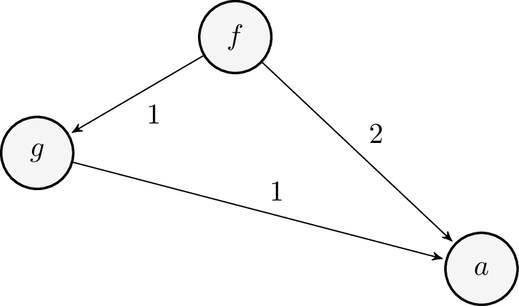
Again, a bottom up strategy allows us to construct a solution as tuples:
\begin{align*} t_1 &\mapsto {\sf f(g(a), a)}\\ t_2 &\mapsto {\sf g(a)}\\ t_3 &\mapsto {\sf a}\\ \end{align*}In Racket, we would this as
(let* ([t3 (a)]
       [t2 (g t3)]     ; sharing t3
       [t1 (f t2 t3)]) ; sharing t3
  (check-equal? t1 '(f (g (a)) (a))))
It is worth noting that while systems of equations in the above example and Example 6.2, they both result in the same sets of behaviours, i.e., terms. For example, the behaviour \({B}(t_1)\) is identical to that of \(t_1\) in Example 6.2.
8.14.2 Infinite Term Graph
Consider an infinite graph
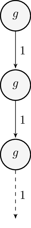
Now it is no longer possible to write the `solution' of \(t_1\) as a finite nested list. Instead, we informally write \(t_1\) to be the term \({\sf g}({\sf g}({\sf g}(\ \ldots )))\).
A more precise semantics of the term at \(t_1\) may be obtained by constructing the behaviour \({B}(t_1)\):
\begin{align*} [\ ] & \mapsto {\sf g}\\ [1] & \mapsto {\sf g}\\ [1\ 1] & \mapsto {\sf g}\\ \vdots \end{align*}Notice that this is also the behaviour of each of the \(t_i\)'s.
8.14.3 Cyclic Term graph
Infinite (or co-inductive) terms can be obtained as solutions to a finite set of equations. Consider the cyclic term graph with one vertex:
\begin{align*} t_1 & \eqn {\sf g}(t_1) \end{align*}
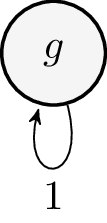
Because of the self-loop, the position space of \(t_1\) is infinite: \([\ ], [1], [1\ 1], \ldots\) . The position space is \(1^*\). Each position \(1^n\) is mapped to the constructor \({\sf g}\). This is identical to the behaviour at vertex \(t_1\) Example 8.14.2.
9 Reasoning about Equality of Terms via Bisimulation
When are two terms the same? Since we identify terms with behaviour, the equality of terms is derived from equality of behaviour. Now, two behaviours are identical if they are equal as functions: they share the same domain of definition and they match for each position in that domain. One problem from a practical standpoint is that the domains of the terms may be large or even infinite.
Another approach is to consider the vertices in a term graph whose solution maps the vertices to the terms we wish to compare. Now we are no longer looking at the terms directly, but through the structural (head and edge) relationships between vertices they represent in a term graph.
We need to be careful in defining what we mean by `same'. Sameness and distinction between objects depends on what we are allowed to observe about the objects. Thus equivalence of objects is modulo `observation.' In the case of terms, the observations are constructor symbols and we are allowed to examine the head of a term to identify the constructor. Now, equal terms should not only have equal heads, but the equality should also hold for the corresponding pairs of subterms. For example, consider the term equations \(t_1 \eqn {\sf f}(t_2, t_3)\) and \(t'_1 \eqn {\sf f}(t'_2, t'_3)\). Suppose we were to claim that \(t_1\) and \(t'_1\) denote the same term. We then need to show that this equality must also `flow down' to the subterms: i.e, we should have equality between \(t_2\) and \(t'_2\) and also between \(t_3\) and \(t'_3\). Let's call this inference rule `DOWN'. We also want equality to flow upwards. So if the corresponding subterms are equal, then clearly the terms constructed with the same constructor and the corresponding subterms should be equal. Let's call this rule `UP.'
9.0.1 Example of circular reasoning
We need to be careful, for, otherwise we could be trapped in a hopelessly circular argument: Consider the term graph with two vertices:
\begin{align*} t_1 & \eqn {\sf g}(t_2)\\ \\ t_2 & \eqn {\sf g}(t_1) \end{align*}We want to show that both the vertices \(t_1\) and \(t_2\) refer to the same infinite term \({\sf g}({\sf g}(...))\). Now, if were to reason using the `DOWN' rule, we end up with something like this:
\(t_1\) are \(t_2\) are the same, because their heads are the same (both are \({\sf g}\)) and their immediate subterms, viz \(t_2\) and \(t_1\) are the same.
This is clearly a circular argument. The objects of our reasoning may be circular, but circular reasoning is mathematically unacceptable: A proof can not assume what it is trying to prove. Trying the `UP' rule instead doesn't help either. A different approach is needed, and this is where the notion of bisimulation comes in.
The intuitive idea behind bisimulation is that we `decree' that two terms are equal, and challenge anyone to show us where we are wrong. This kind of reasoning may seem untenable, but it's not without value or use. Imagine a court scene in which a defendant charged with murder claims that he was away with his friend in Mumbai on the night of a crime that took place in Delhi. His alibi provides an argument consistent with the defendant's claim. Should the defendant be pronounced guilty? In the absence of any contradictory evidence challenging or repudiating the claims of the defendant, a jury will be unable to prosecute the defendant and the defendant will be acquitted.
Reasoning with bisimuation is similar: first we propose an `equality' (bisimulation) relation. Then, we try to verify that this relation is consistent with the equality flowing down between subterms.
9.1 Definition of Bisimulation
Let \(T\) be a \(\Sigma\)-term graph with vertex set \(V\). A relation \(R\subseteq V\times V\) is a bisimulation if for each pair \((v,v')\in R\), the following is true:
- \(\id{h}(v)=\id{h}(v')\): Their heads are the same, and
- for each \(i\), \(1\leq i \leq \alpha(\id{h}(v))\), if \(v\xto{i}{}v_i\) and \(v'\xto{i}{}v'_i\), then \((v_i, v'_i) \in R\).
We say two vertices \(v\) and \(v'\) in the $Σ$-term graph are bisimilar iff there is a bisimulation relation \(R\) such that \((v,v')\in R\).
Therefore, we work with bisimilarity as the notion of observational equivalence between vertices. One way of thinking about this (and it will be generalised in later classes) is that vertices are like `states': black boxes that allow only specific observations about them and interactions that take you to other vertices. Vertices that are bisimilar have the same observations. In addition, identical interactions with them take us to states that are themselves bisimilar.
9.2 Examples
9.2.1 Reasoning about equality based on induction
Consider the terms in Examples 6.2 and 8.14.1. If we take a larger term graph that include both of the individual term graphs and rename the vertices in Example 8.14.1 with primes, then we want to show that vertices \(t_1\) and \(t'_1\) refer to the same term. Since both these term graphs are acyclic, we can proceed by reasoning with induction. We define equality inductively via the judgement \(t \sim_{\sf ind} t'\).
\begin{align*} \frac{t_1 \sim_{\sf ind} t'_1, \ldots t_n \sim_{\sf ind} t'_n}{t\sim_{\sf ind}t'}\quad t=f(t_1, \ldots, t_n)\ \text{and}\ t'=f(t'_1, \ldots, t'_n) \qquad \qquad UP \end{align*}Exercise: Using this rule, we prove that \(t_1 \sim_{\sf ind} t_2\).
As mentioned earlier, this rule is useless in the presence of circular or infinite term graphs; instead, we need reasoning based on bisimulation.
9.2.2 Reasoning about equality based on bisimulation, or co-induction
Consider again the graphs in Examples 8.14.2 and 8.14.3 (with the vertex in Example 8.14.3 primed so as to be distinguishable from those in Example 8.14.2. We would like to show that all the vertices in the two term graphs are bisimilar to each other. For this, we construct a bisimulation relation
\[R = \set{(t_i, t'_1)} \ |\ i\in \N_1\]
We claim \(R\) is a bisimulation. To prove this, we pick an arbitrary pair \((t_i, t'_1)\) from \(R\). Clearly, \(t_i\) and \(t'_1\) have the same head, viz., \({\sf g}\). Now, \(t_i\xto{1}{}t_{i+1}\) whereas \(t'_1\xto{1}{}t'_1\). We need to verify if the pair \((t_{i+1}, t'_1)\) is in \(R\). It is, because that's how we chose \(R\) in the first place! Therefore, \(t_1\) and \(t'_1\) are bisimilar. As you can see, establishing bisimilarity hinges on guessing an appropriate bisimulation relation and sometimes that could take some effort.
Consider now the Example 9.0.1. Here the bisimulation \(R=\set{(t_1, t_2)}\) is sufficient to witness the bisimilarity of \(t_1\) and \(t_2\).
10 Replacement
In the model of computing that we are interested in this course, computation proceeds by reducing term trees. The reduction operation relies on replacement: taking a term tree, identifying a subtree and replacing that subtree with another term tree.
We will try to understand replacement in the more general setting of term graphs.
10.1 Replacement
Let \(G\) be a term graph and let \(t\) be a term vertex and let \(t_p\) be the subterm vertex of \(t\) at position \(p\). Let \(s\) be another term vertex. If we think of \(t\) as the root of a a (possibly infinite) tree, then the replacement of the subterm of \(t\) at position \(p\) by term \(s\), denoted \(\id{replace}(t,p,s)\) results in a new term graph. Everything works out nicely when the terms are inductive or infinite. But, when dealing with circular term graphs, `unrolling' the circular term graph is necessary when performing replacement.
Here are some examples. For replacement involving term trees, we dispense with writing down elaborate term graphs and rely on the tree (expression) notation:
\begin{align*} \id{replace}({\sf f(g(a), b)}, [1\ 1], {\sf b}) = {\sf f(g(b), b)}\\ \\ \id{replace}({\sf f(g(a), b)}, [1], {\sf b}) = {\sf f(b, b)}\\ \\ \id{replace}({\sf f(g(a), b)}, [\ ], {\sf b}) = {\sf b} \end{align*}What happens when (sub)terms are shared? Consider
\begin{align*} t_1 &\eqn {\sf f}(t_2, t_3)\\ t_2 &\eqn {\sf g}(t_3)\\ t_3 &\eqn {\sf a}\\ t_4 &\eqn {\sf b} \end{align*}What is the result of \(\id{replace}(t_1, [1\ 1], t_4)\)? Is it \({\sf f(g(b), a)}\) or \({\sf f(g(b), b)}\)? The correct answer is \({\sf f(g(b), a)}\) because we may think of position \([1\ 1]\) as a pointer which is now pointing to \(t_4\). The pointer \([2]\) is unchanged.
10.1.1 Example: replacement involving cycles
Now consider the following situation that involves cycles in the term graph:
\begin{align*} t_0 &= {\sf g}(t_0) \end{align*}Here, the term graph consists of a single vertex \(t_0\) pointing to itself, denoting the infinite term \({\sf g(g(g(\ldots)))}\). Suppose we wish to replace in \(t_0\), the subterm at position \([1\ 1]\) with the term \(s={\sf a}()\). Then, we first need `unroll' \(t_0\) a sufficient number of times before we can graft \(s\) at the right position.
\begin{align*} t_0 &={\sf g}(t_1)\\ t_1 &={\sf g}(t_2)\\ t_2 &={\sf a}() \end{align*}10.2 Defining subterm and replacement
Let \(t\) be a term and let \(p\) be a position in \(t\). Let \(t'\) be a subterm of \(t\) at position \(p\). This means that
- \(p\in \id{pos}_G(t)\).
- If \(q\in \id{pos}_G(t')\), then \(pq\in \id{pos}_G(t)\) and \(t(pq) = t'(q)\).
Let \(s\) be a term. \(\id{replace}(t, p, s)\) results in the following term \(r\):
\begin{align*} \id{pos}_G(r) &= (\id{pos}_G(t) \setminus \set{a\in\id{pos}_G(t) |\ \id{prefix}(a)=p}) \\ &\union \set{p}\id{pos}_G(t') \end{align*}We define \(r\) via pattern matching positions:
\begin{align*} r (pq) &= s(q) & \text{for each}\ pq\in \id{pos}_G(r)\\ r (q) &= t(q) & \text{if $p$ is not a prefix of $q$}\\ \end{align*}Exercise: Verify that the result of a replacement is indeed a term.
10.2.1 Example
Consider again Example 10.1.1. The term graph \(t_1={\sf g}(t_1)\) yields the following term: \(\set{(1^n\mapsto {\sf g})\ |\ n\in \N}\). The term \({\sf a}()\) corresponds to the term \(\set{[\ ]\mapsto {\sf a}}\). Replacing the subterm at position \([1\ 1]\) in \(t_1\) with with \({\sf a}()\) yields the term \(r\). The position space of is \(\set{[\ ], [1], [1\ 1]}\).
\begin{align*} r\ [\ ] &= {\sf g}\\ r\ [1] &= {\sf g}\\ r\ [1\ 1] &={\sf a} \end{align*}11 Implementing term graphs and replacement in Racket
The following Racket implmentation tries to capture the idea of co-inductive terms and replacement. We do not explicitly need to construct a representation of behaviour functions or term graphs. These happen behind the scenes in the implementation. The racket implementation provides a `user-interface' to build inductive and co-inductive terms.
11.1 Inductive term
We define inductive terms as lists whose first element is a
symbol. For simplicity we will altogether avoid arity
checking. Every time we call list a brand new vertex is
created in the term graph.
(check-true (term? (list 'a)))
(check-true (term? (list 'g '(a))))
(check-true (term? '(f (g (a)) (a))))
11.2 Co-Inductive terms
To define co-inductive terms, we need a co-inductive version
of list: colist.
(check-true (term? (list 'g '(a))))
(check-true (term? (colist 'g '(a))))
(check-true (term? (rec t (colist 'g t))))
(check-true (term? (list 'g (rec t (colist 'g t)))))
colist is defined by extending Racket's syntax. colist
is a lazy constructor. It does not evaluate its arguments,
and thereby allows delaying their evaluation. This is a
crucial tool to construct co-inductive terms. We have
already seen a cousin scons of colist which was used to
construct streams.
(define-syntax colist
  (syntax-rules ()
    [(colist sym terms ...)
     (lambda () (list sym terms ...))]))
A term is either one built inductively (using list) or
built co-inductively (using colist):
;;; term? :: any/c -> boolean?
(define term? (or/c procedure? list?))
The head of a term returns the constructor:
(check-equal? (hd (g (a))) 'g)
(check-equal? (hd (rec t (colist 'g t))) 'g)
If the term is a list, that's easy: the head is just the
car of the list. If the term is built using colist,
then we will need to first unroll the procedure representing the
term to get a list. Then we take the car of that list.
;;; unroll :: term? -> term?
(define (unroll t)
  (if (procedure? t) (t) t))

;;; hd :: term? -> symbol?
(define (hd t)
  (car (unroll t)))
11.3 Index
An index is a positive integer.
;;; posint? :: any/c -> boolean?
(define posint? (and/c integer? (>=/c 1)))
(define index? posint?)
11.4 Term reference
Now that we have the head, let's try to locate the children
of a term. Analogous to Racket's list-ref, we define
term-ref ,which returns the i=th element of the (list
representing) the term. =term-ref indexes into a term and
returns the immediate subterm at that index. If the index
is greater than the arity of the term's head, Racket throws
an error.
;;; term-ref :: term? posint? -> term?
(define (term-ref t i)
  (list-ref (unroll t) i))

(check-equal? (term-ref (list 'f '(a) '(b)) 1) '(a))
(check-equal? (term-ref (list 'f '(a) '(b)) 2) '(b))
(check-exn exn:fail? (lambda () (term-ref (list 'f (a) '(b)) 3))) ; index type checking
11.5 Position
A position is a sequence of indices.
;;; pos? :: any/c -> boolean?
(define pos? (listof index?))
(check-true (pos? '()))
(check-true (pos? '(1 3 2)))
(check-false (pos? '(0 1)))
11.6 Subterm
Given a position pos in a term t we want to find the subterm at
that position.
(check-equal? (subterm '(f (a) (a)) '())
              '(f (a) (a)))

(check-equal?  (subterm '(f (a) (b)) '(2))
              '(b))

(letrec ([t (colist 'g t)])
  (check-equal?  (subterm  t '(1 1))
                 t))


(letrec ([t (colist 'f t '(a))])
  (check-equal? (subterm t '(1 1 2))
                '(a))
  (check-equal? (subterm t '(1 1 1))
                t))
If the position is empty, then the answer is
t. Otherwise, we take the first index from pos, say i,
and search inside the i=th child t_i of t.
;;; subterm :: term? pos? -> term?
(define (subterm t pos)
  (letrec ([loop (lambda (t pos)
                   (cond [(null? pos) t]
                         [else (let* ([i (first pos)]
                                      [t_i (term-ref t (first pos))])
                                 (loop t_i (rest pos)))]))])
    (loop t pos)))
11.7 Replacement in a flat list
Before defining replacement in terms, we consider a simpler
situation: replacing an element at a particular index in a
list with another element. We call this operation
replace-flat. (replace-flat ls i val) takes a list
ls, an index i within the boundaries of ls and a value
val and return a new list whose value at position i is
val, but all other positions, it is the same as that of
ls.
(check-equal? (replace-flat '(f a b) 1 'c) '(f c b))
(check-exn exn:fail? (lambda ()  (replace-flat '(f a b) 0 'c)))
11.7.1 replace-flat definition
replace-flat checks if i is a sane value. If so, it
calls replace-flat-helper, otherwise it raises an error.
replace-flat-helper is a simple exercise in list
recursion.
;;; replace-flat :: list? index? any/c -> list?
(define (replace-flat ls i val)
  (if (and (posint? i)
           (<= i (length ls)))
      (replace-flat-helper ls i val)
      (error 'replace-flat "incompatible args: ls: ~a, i:~a" ls i)))

(define (replace-flat-helper ls i val)
  (letrec ([f (lambda (l j)
                (cond [(zero? j) (cons val (cdr l))]
                      [else (cons (car l)
                                  (f (cdr l) (sub1 j)))]))])
    (f ls i)))
11.8 Replace
Now we come to replace.
In the first test below, the subterm (a) in the term (g
(a)) occurs at position [1] and is replaced (b).
(check-equal?  (replace '(g (a)) '[1] '(b))
               ;; replace '(a) with '(b)
               '(g (b)))
In the test below, the subterm (a) occurs at position [1
1] in the top level expression and is again replaced by
(b).
(check-equal?  (replace '(f (g (a)) (b)) '[1 1] '(b))
               ;; replace (a) with (b)
               '(f (g (b)) (b)))
In the test below, a coterm t is constructed as shown
below in Figure 5 on the . We wish to
replace the subterm at position [1 1 2] in t with
(b). That involves unrolling t a few times before
(b) can be grafted at the position [1 1 2]. The result
is shown in Figure 6.
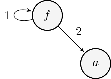
Figure 5: Term t (root)
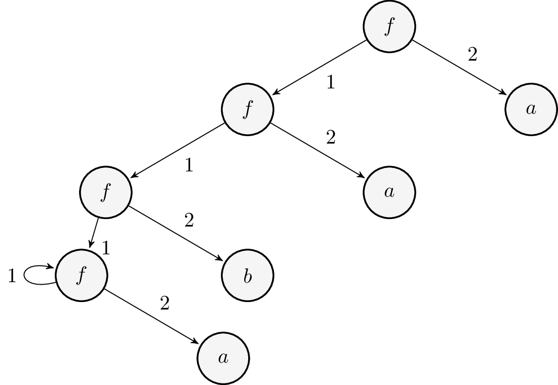
Figure 6: Replacing t's subterm at [1 1 2] with '(b)
(letrec ([t (colist 'f t '(a))])
  (let ([r (replace t '[1 1 2] '(b))])
    (check-equal?  (subterm r '[1 1 2]) '(b))
    (check-eq? (subterm r '[1 1 1]) t))) ; this last test should get you thinking!
Exercise: Write systems of flat equations that precisely mimic the term graphs according to the Racket implementation. Then, draw diagrams of other possible term graphs that represent the replacement.
11.8.1 Implementing replace
replace takes a term t, a position pos and a graft
term.
- If the position is null, we return the graft.
- Otherwise, we locate the immediate subterm of
tat(car pos), sayti. We replacetiwith thegraftat position(cdr pos). Let the result bes. - Finally, we
replace-flattwithsat position(car pos).
;;; replace: term? pos? term? -> term?
(define (replace t pos graft)
  (let ([t (unroll t)])
    (cond [(null? pos) graft]
          [else (let* ([ti (term-ref t (car pos))]
                       [s (replace ti (cdr pos) graft)])
                  (replace-flat t (car pos) s))])))
11.9 Boilerplate
#lang racket
(require racket/contract)
(require racket/list)
(require rackunit)
(require mzlib/etc)
(provide (all-defined-out))
12 Implementing Bisimulation for Rational terms
In the Racket test cases below, each test below correctly describes the bisimilarity of the given terms.
Exercise: Draw the graphs representing each of the systems represented in the test cases. Convince yourself that these test cases make sense.
12.1 Test cases
(let ([t (a)])
  (check-true (bisimilar? t t)))

(let ([t1 (colist 'a)]
      [t2 (list 'a)])
  (check-true (bisimilar? t1 t2)))

(letrec ([t (colist 'g t)])
  (check-true (bisimilar? t t)))

(letrec ([t (colist 'g t)])
  (check-true (bisimilar? t (subterm t '[1 1]))))

(let* ([t1 (a)]
       [t2 (a)])
  (check-true (bisimilar? (list 'f t1 t2) (list 'f t1 t1))))

(letrec ([t1 (colist 'g t2)]
         [t2 (colist 'g t1)])
  (check-true (bisimilar? t1 t2)))


(letrec ([t1 (colist 'g t2)]
         [t2 (colist 'g t2)])
  (check-true (bisimilar? t1 t2)))
12.2 Implementation
Exercise: Implement the function bisimilar?.
13 References
13.1 Induction
- Ana Bove 2018
- Notes on Inductive Sets and Induction.
13.2 Co-Induction
- Kozen and Silva, 2016. Practical Co-Induction
- Math. Structures in Computer Science. pp 1–21. 10.1017/S0960129515000493.
- Bahr 2012
- Infinitary Term Graph Rewriting is Simple Sound and Complete. Rewriting Techniques and Applications. 2012
- Co-inductive Foundations of Infinitary Rewriting and Infinitary Equational Logic
- Endrullis et al. Logical Methods in Computer Science. Vol 14(1:3) 2018 pp. 1–44. http://www.lmcs-online.org
13.3 Knaster Tarski Theorem
- Wikipedia page on Knaster-Tarski Theorem
- Online Notes.
- Cornell CS 6110 S 17 Lec 7 Notes
13.4 Solution Lemma and non-well-founded set theory
- Moss, Lawrence S. 2018
- Non-wellfounded Set Theory, The Stanford Encyclopedia of Philosophy (Summer 2018 Edition), Edward N. Zalta (ed.),
- Akman and Pakkan, 1996
- Nonstandard set theories and information management. A readable discussion of Set Theory with the Anti-foundation axiom and its application to relational database theory (Sec 3.2).